1. Dynamics of buoyancy-driven eastern boundary currents
2. Interannual variability of the Gulf Stream position
3. Transport by coherent mesoscale eddies
4. Free motion on a parabolic dish

---

[top]

---

Dynamics of Buoyancy-Driven Eastern Boundary Currents

With Suyash Bire (Ph.D. Student)
Funding: National Science Foundation

• Most eastern boundary currents are driven by local winds and flow toward the equator.
• The Leeuwin Current off Western Australia flows opposite to the wind and is driven by the large-scale buoyancy gradient in the Indian Ocean.
  • Most wind-driven eastern boundary currents have poleward undercurrents which may be similarly buoyancy driven.

Mechanism for buoyancy driven eastern boundary currents

• Surface waters are cooler and denser at high latitudes than low latitudes
• This density gradient drives a vertically sheared zonal flow via thermal wind, with eastward flow at the surface.
• Downwelling at the coast displaces isopycnals, setting up a geostrophically balanced poleward current.
• The current eventually becomes unstable, radiating waves and eddies which dissipate the cross-shore density gradient.
• Question: Why isn’t the density gradient entirely destroyed? Why is the current there at all?
• Approach: Idealized, process-oriented modeling study using an isopycnal coordinate model (MOM6) at high resolution.
• We are currently diagnosing momentum and vorticity balances to determined the mechanism which traps the eastern boundary current near the coast.

This animation surface vorticity (colors) and sea surface height (shading) from year 17 of a reference simulation. The warm eastern boundary current is visible at midlatitudes near the coast (0º longitude). The eastern boundary current sheds warm-core, anticyclonic eddies (blue patches). These eddies transport negative vorticity from the boundary and the resulting build-up of positive vorticity near the coast sharpens the boundary current.

[top]

---

Interannual Variability of the Gulf Stream Position

With Sultan Hameed (SoMAS) and Lequan Chi  (Ph.D. Student)
Funding: National Science Foundation

• The Gulf Stream North Wall (GSNW) divides warm, salty subtropical waters from the colder, more productive shelf and slope waters.
• Gulf Stream meanders on intraseasonal and longer time scales.
• Interannual shifts in the GSNW affect local climate (northward shifts are associated with increased storminess), European climate, and local fisheries.
• GSNW influenced by the North Atlantic Oscillation (NAO), particularly the position and strength of the Icelandic Low.
• Details of the NAO’s influence are not fully understood, such as
  • How does the NAO influence in GSNW?
  • How long does it take?
  • It is really the NAO, is the Icelandic Low the primary actor?

We are attempting to answer questions with a three pronged approach:

1. Statistical analysis of observations
2. Dynamical analysis of 3D data from ocean reanalyses
3. Perturbation experiments using ocean models

A major effort in support of prong (2) is the evaluation of the available ocean reanalysis to determine which (if any) has a “good” representation of the Gulf Stream. HYCOM (shown above), with a resolution of approximately 1/12º, tends to do quite well. (See Taylor diagram below). However, HYCOM uses a sequential assimilation procedure and these violate the basic conservation laws of fluid motion. ECCOv4, a state estimate which respects conservation laws to numerical precision, has a surprisingly realistic Gulf Stream, despite its coarse resolution. Most other reanalyses have Gulf Stream variability which is several times the amplitude, and uncorrelated with, the observations.

[top]

---

Free Motion on a Parabolic Dish

Background

Inertial oscillations—motions with periods near the inertial period—are ubiquitous in the ocean. Despite being textbook material, their dynamics are often misunderstood. In particular, since particles undergoing inertial oscillations do not follow straight lines in an inertial frame far from Earth, the ‘inertial’ nature of inertial oscillations has been questioned. Early (2012) showed that the motion tangent to the surface of the Earth is indeed inertial—an accelerometer executing inertial oscillations would only record accelerations normal to the surface of the Earth.

While Early’s arguments are compelling, demonstration of the inertial nature of inertial oscillations is challenging due to the large space and time scales necessary for the Coriolis effect to significantly affect motion on the Earth. If a dish is filled with resin or molten glass and allowed to harden while rotating, the parabolic dish becomes a hard rotating surface upon which the tangential components of gravity and centrifugal acceleration cancel. Thus, the parabolic dish provides a laboratory analog for the surface of the rotating Earth and free motion of a particle on this dish provides an ideal laboratory model for inertial oscillations. (This is used to great effect in MIT’s Weather in a Tank module.)

Current Work

We have found exact solutions for free motion on a parabolic dish with arbitrarily large curvature. These solutions allow examination of richer dynamics than possible with those derived assuming the that parabola’s curvature is weak. A few interesting dynamical regimes are illustrated below.

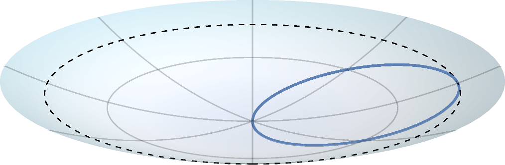
Zero angular momentum oscillations

Laboratory Frame	Co-rotating Frame

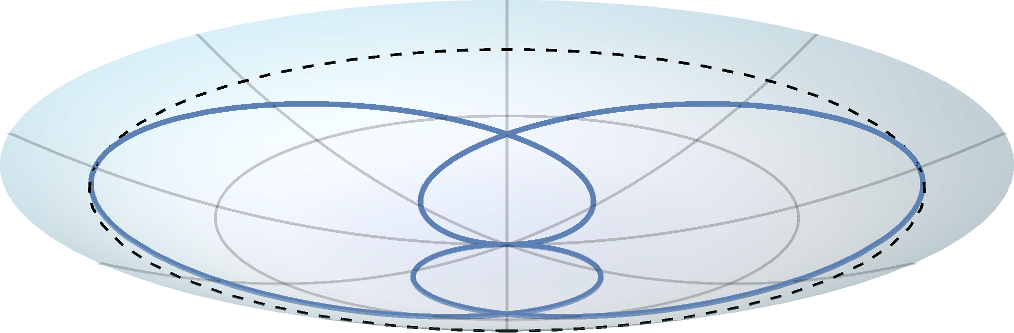The particle passes through the center of the dish if its angular momentum is zero. The trajectory appears as a straight line in the laboratory frame, but appears to bend under the Coriolis force in a frame co-rotating with the dish. For infinitesimally small curvatures (top row), the rotation period is exactly twice the oscillation period, so the particle appears to make two closed loops in the rotating frame for every back-and-forth oscillation in the laboratory frame. For finite curvatures (bottom row), the period is longer than the oscillation period. The figures are still closed if the rotation period is a rational multiple of the oscillation period, but the particle performs extra loops before closing the path.

Oscillations about a circular orbit

Suppose the particle is initially at rest in the rotating frame at radius R. The particle is then accelerated with an impulsive force that gives it an initial inward velocity.

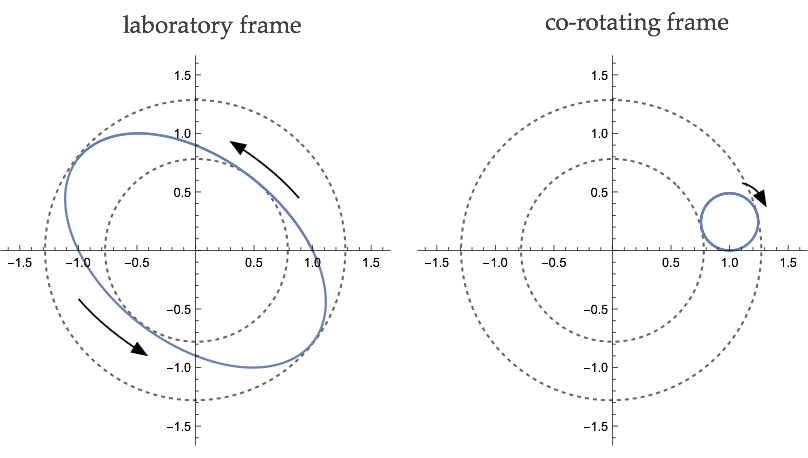
For infinitesimal curvatures, the new orbit is elliptical in the laboratory frame. In the co-rotating frame, the particle appears to execute a smaller circular orbit in the opposite direction. This is a classical inertial oscillation.

The elliptical orbit precesses in the fixed frame for finite curvatures, leading to highly braided trajectories. The precession in the fixed frame is expressed as a slight distortion and drift of the original inertial circle in the direction opposite to the sense of the overall rotation. This drift is analogous to the westward drift of inertial circles on the Earth under the influence of the β-effect.

[top]