Grover’s Algorithm was developed by Lov Grover as a quantum search algorithm designed to only need \(O(\sqrt{N})\) runtime in contrast to classical search algorithm’s which require \(O(N)\).

The idea behind Grover’s algorithm is to first use an oracle to mark the correct answer by applying a negative to the correct answer. This oracle utilizes superposition to mark the correct answer. It essentially checks the input to see if it is the “correct answer” (the item that the algorithm is searching for) and if it is, it changes the amplitude to negative.

The simplest example to understand this is Grover’s algorithm running on a two-qubit system searching for ’11’ (I will address the circuits for the other three combinations at the end of the page). The gate solely consists of a control-Z gate.

A control-Z gate is just a CNOT gate with two Hadamard gates (one before and one after) the target qubit. It is also represented by this:

This is important to understand because in IBM Q’s Grover Algorithm page, they use the H-cNOT-H gate as the oracle, whereas I just used Jupyter’s cZ gate. They are the same; just the cZ gate is easier. Also, for future reference, you will be able to recognize the cZ gate if given a circuit including the H-cNOT-H gates.

Anyways, so how does this cZ gate even mark the amplitude of \(|11\rangle\) negative? To answer this, we can look at the matrix for the cZ gate: \(cZ = \begin{bmatrix}
1 & 0 & 0 & 0 \\
0 & 1 & 0 & 0 \\
0 & 0 & 1 & 0 \\
0 & 0 & 0 & -1 \\
\end{bmatrix}\)

This 4×4 matrix actually represents the amplitudes of all the different basis of the 2-qubit system.

To read this matrix, you can see the initial state on the horizontal axis and then the ending state on the vertical axis. For example, if the matrix \(cNOT = \begin{bmatrix}
1 & 0 & 0 & 0 \\
0 & 1 & 0 & 0 \\
0 & 0 & 0 & 1 \\
0 & 0 & 1 & 0 \\
\end{bmatrix}\) you can clearly see that 10 is mapped to 11 and 11 is mapped to 10. This makes sense for a cNOT gate; if the first qubit is 1 then the value of the next qubit is flipped.

In the cZ gate scenario, however, all values are mapped back to themselves; the only difference is that \(|11\rangle\) now has a negative amplitude.

Okay, so where to now? How does this negative amplitude correlate to finding \(|11\rangle\)? I will introduce a purely visual helping tool; I had a lot of difficulty with this picture as I kept on trying to draw connections between the image and the physical qubits.

Firstly, the vertical \(|\beta\rangle\) axis is the “solutions axis” — the closer the vector is to that axis, the higher the probability that the qubits will be the correct solution. Now, when the qubits are just in equal superposition, they are represented by the vector \(|\psi\rangle\). As you can see, the vector is quite close to the \(|\alpha\rangle\) axis which is the “non-solutions” axis, because there are more solutions than non-solutions in our case. For simplicity, I will always assume that there is only one solution and the rest are non-solutions.

So for a two-qubit system, searching for \(|11\rangle\) means a \(\frac{1}{4}\) chance when the qubits are in an equal superposition (equal probability of the results being \(|00\rangle\) or \(|01\rangle\) or \(|10\rangle\) or \(|11\rangle\)).

The oracle, represented by \(O\) applies the negative to the correct answer and thus the vector is now under the \(|\alpha\rangle\) axis. Keep in mind that its amplitude still has a magnitude of 1 and thus there is still an equal probability of it being any of the four possible answers. To understand this visually, just understand that the \(|\beta\rangle\) axis extends downwards too — it is not just the 1st quadrant — as well as the \(|\alpha\rangle\) axis extends to the left too.

The next part of Grover’s algorithm reflects the vector \(O|\psi\rangle\) across \(|\psi\rangle\) to \(G|\psi\rangle\) and assuming that the original vector’s angle was \(\frac{\theta}{2}\), then the original vector was rotated \(\theta\) towards the \(|\beta\rangle\) axis to get to \(G|\psi\rangle\).

To reflect \(O|\psi\rangle\) across \(|\psi\rangle\), we must use the inversion about the mean operator which is the next part of Grover’s algorithm. If you click here and look at the right-hand side picture of step 1 to step 2, it will give a visual representation of what we are doing. There is a formula for this: \(2|\psi\rangle\langle\psi|-I\) which is also sometimes represented as \(2|s\rangle\langle s|-1\). The decomposition of this is \(H^{\otimes n}(2|0\rangle\langle 0|-I)H^{\otimes n}\), where \(H^{\otimes n}\) just signifies Hadamard gates on all the cubits. \(2|0\rangle\langle 0|-I\) in the quantum circuit is represented by:

I will explain why this is the case a little farther down, just trust me for now. Thus, the entire reflection circuit is

This whole thing was a single Grover’s iteration: the oracle then two reflections. However, as \(\theta\) becomes smaller, more and more rotations are needed, so how many rotations are needed? Well, for a two-qubit system, only one rotation is needed to get \(|\psi\rangle\) exactly to \(|\beta\rangle\). With some other qubits, however, it may not be as precise. Furthermore, we need to ensure that we do not go too far past the vertical axis or else it’ll be closer to the non-solutions yet again. To find \(\theta\), the formula is $$sin(\theta) = \frac{2\sqrt{M(N-M)}}{N}$$
In this formula, M is the number of solutions and N is the total number of possibilities (solutions + non-solutions). There is a very good proof for this in chapter 6.1 of the book: Quantum Computation and Quantum Information by Nielsen and Chuang. But, don’t sweat it if you can’t access it, just know that that is the formula.

Using that formula, \(\theta\) can be calculated to be \(\frac{\pi}{3}\) and since \(\frac{\theta}{2}\) would be \(\frac{\pi}{6}\), a single rotation would bring \(|\psi\rangle\) to \(\frac{\pi}{2}\) which is \(|\beta\rangle\).

Furthermore, Nielsen and Chuang introduce another formula $$R \leq \lceil\frac{\pi}{4}\sqrt{\frac{N}{M}}\rceil$$ where R is the maximum integer number of rotations needed to rotate close to \(|\beta\rangle\).

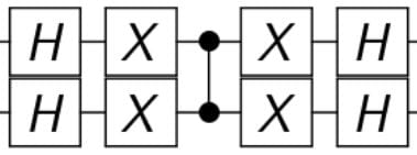
So, for the two-qubit Grover’s algorithm, there are three other possibilities we currently do not have an oracle for (the reflection is always the same). But, if we think about this logically (an ingenious solution presented by Dr. Tzu-Chieh Wei — my mentor if you didn’t know) was utilizing X gates both before and after. For example, if we have the cZ gate and put two X gates on qubit 0 and qubit 1 both before and after, the cZ gate will change the amplitude of 00 to negative. This is because the cZ gate changes the amplitude to negative only if the input is 11. So clearly, two X gates would result in the amplitude becoming negative only if the input is 00. We can manipulate this to the other two possibilities to get the gates necessary to get ’01’ and ’10’.

But, you recognize two X gates with a cZ gate in the middle right? It is the \(2|0\rangle\langle 0|-I\) inversion about the mean operator. That makes sense, though. Because \(|0\rangle\) is represented by \(\begin{bmatrix}
1 \\
0 \\
0 \\
.. \\
\end{bmatrix}\) depending on how many qubits there are and \(\langle 0|\) is represented by \(\begin{bmatrix}
1 & 0 & 0 & .. \end {bmatrix}\).

So multiplying them together and then by 2 would yield \(\begin{bmatrix}
2 & 0 & 0 & .. \\
0 & 0 & 0 & .. \\
0 & 0 & 0 & .. \\
.. & .. & .. & .. \\
\end{bmatrix}\).

Lastly, subtracting \(I\) gives

\(\begin{bmatrix}
1 & 0 & 0 & .. \\
0 & -1 & 0 & .. \\
0 & 0 & -1 & .. \\
.. & .. & .. & .. \\
\end{bmatrix} = -\begin{bmatrix}
-1 & 0 & 0 & .. \\
0 & 1 & 0 & .. \\
0 & 0 & 1 & .. \\
.. & .. & .. & .. \\
\end{bmatrix}\). Also, the negative sign in front of the matrix is effectively irrelevant.